The Fifth Percentile, or an "Arbitrary Choice"
How a round number came to set limits for pollutants in rivers and soils



This essay is part of a series on the origins of the principles of regulatory toxicology. We have traced the 100-fold safety factor (Of Mice and Men and Round Numbers), the one-in-a-million cancer risk (One in a Million) and the claim that some chemicals in food need not be tested at all (De Minimis, or "Sheer Nonsense").
Here we turn to how regulators decide how much of a pollutant is safe in rivers or soil. The widely used method is called the species sensitivity distribution, or SSD. Researchers test a chemical in the laboratory on a set of species, usually eight to a few dozen (though for one recent compound, as we show below, the limit was based on tests in just two species). They then fit a statistical distribution to the results and estimate the concentration that would harm 5 percent of species. That concentration, often divided by a small safety factor, becomes the limit. Regulators assume this protects the other 95 percent of species. This method sets limits for pollutants in water in the United States, the European Union, Australia and elsewhere, and for soil in the Netherlands.
Some see methods like this as too cautious, setting limits far below any demonstrated harm. The same complaint was made about the rules discussed in our earlier essays (One in a Million; De Minimis), and it has been made about SSDs (Solomon et al., 2000; Versteeg et al., 1999). Others may see the SSD as reckless: a curve fitted to a handful of laboratory species is used to permit pollution of ecosystems that are poorly understood and hard, sometimes impossible, to repair (Smetanová et al., 2014; US EPA SAB, 2006).
The 5 percent figure itself did not come from a deliberate calculation. The US EPA chose it in 1985 because other values gave results that "seemed too high or too low" (US EPA, 1985). The Dutch scientists who chose it in 1989 entered its basis in their table as "Arbitrary choice," and the Dutch cabinet adopted it "for the time being" (van Straalen & Denneman, 1989; VROM, 1989). In both countries the number was kept because the limits it produced looked reasonable. At a 1990 workshop the SSD method got its name, and a list was drawn up of what still had to be checked. Though first framed as work in progress, the method has changed little in thirty-six years and its initial assumptions have become the default. Few of those checks were ever carried out, and where researchers did look at real streams, animals were often already declining at concentrations below the calculated safe limit.

The American origin
In 1965 the US Congress passed the Water Quality Act. It required states to adopt water-quality criteria that took into account "propagation of fish and wildlife" as well as "agricultural, industrial, and other legitimate uses" (Water Quality Act, 1965). Two scientists at the federal water-pollution agency in Cincinnati, Donald Mount and Charles Stephan, wrote that the new law "suggests that some type of 'standards' will be forthcoming in the near future" (Mount & Stephan, 1967).
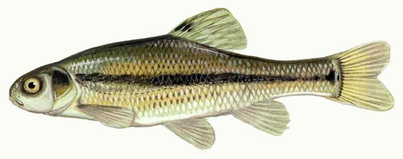
To start developing such standards, Mount and Stephan raised fathead minnows through full life cycles while dosing them with two pesticides. Growth and reproduction were unharmed at 1/45 of the four-day lethal concentration for malathion, and at 1/19 of the four-day lethal concentration for a form of the herbicide 2,4-D. They proposed that such fractions, called application factors, could be applied to other species. They also recognized the limits of laboratory work: its results "should be verified when possible by field observations" (Mount & Stephan, 1967).
In 1976 the settlement of a lawsuit brought by the Natural Resources Defense Council required the US Environmental Protection Agency (EPA) to publish criteria for "65 specified toxic pollutants" (US EPA, 1978).
In 1978 the EPA's draft guidelines proposed limits that would protect "a specified percent of aquatic species," leaving "the policy decision as to how protective the criteria should be" to be made separately (US EPA, 1978). Because no one can test every species, protecting a chosen percentage of them meant treating the tested ones as a sample, and thus extrapolating using a statistical approach. The draft used 95 percent only as an example. The 1980 version calculated the 0.05 point, the fifth percentile, directly from the data for each pollutant (Stephan, 2002). Mount put the reasoning this way in 1982: "each species we test is not representative of any other species but is one estimate of the general species sensitivity" (Suter, 2002).
The method was finalized in 1985. The EPA's Guidelines for Deriving Numerical National Water Quality Criteria call for acute tests (short tests, usually two to four days long) on species from at least eight taxonomic families. The guidelines set the key value, the Final Acute Value, at the concentration "corresponding to a cumulative probability of 0.05," estimated from the four genera (groups of closely related species) that rank closest to that point (in practice almost always the four most sensitive) (US EPA, 1985). The 0.05 means that, on a curve drawn through those four genera, only 5 percent of genera would have an acute toxicity value (typically the concentration that kills or immobilizes half the animals in the test, the LC50 or EC50) lower than the Final Acute Value. The guidelines explain why they do not try to protect every species: "Because aquatic ecosystems can tolerate some stress and occasional adverse effects, protection of all species at all times and places is not deemed necessary." And their reason for choosing 0.05:
The small fraction is set at 0.05 because other fractions resulted in criteria that seemed too high or too low in comparison with the sets of data from which they were calculated. (US EPA, 1985)
In his 2002 account, Stephan added a second reason: "Of the numbers available between 90 and 99, 95 is near the middle and is an easily recognizable number" (Stephan, 2002).
The Dutch origin
The Dutch Soil Protection Act of 1986 called for reference values for contaminants in soil. Cadmium was a concern at the time: in the Kempen, on the Belgian border, metal factories had polluted some 350 square kilometres of soil with cadmium and zinc (Copius Peereboom-Stegeman & Copius Peereboom, 1989). Two ecologists at the Free University in Amsterdam, Nico van Straalen and C. A. J. Denneman, judged the reference values the ministry suggested "as yet, insufficiently based on ecotoxicological evidence," and in 1989 set out to derive their own (van Straalen & Denneman, 1989).
They turned to a new method. In 1987 Bas Kooijman, a theoretical biologist at TNO (the Netherlands Organisation for Applied Scientific Research) in Delft, had published "A safety factor for LC50 values allowing for differences in sensitivity among species." He wanted a concentration that would protect the most sensitive species in a community, and was uneasy about the task:
All honest scientific research workers will feel rather uncomfortable with such a task, and the author is no exception. This feeling finds its roots in the extrapolation of experimental findings far beyond the limits of our knowledge. (Kooijman, 1987)
Van Straalen and Denneman had reproduction data for seven species of soil animals, mostly from published studies: three earthworms, a snail, a woodlouse, a mite and a springtail. Kooijman's method treats every species in the soil, tested or not, as a random draw from one bell-shaped curve. Their sensitivities "can be conceived of as independent random trials from a log-logistic distribution" (Kooijman, 1987). So the two ecologists fitted such a curve to their seven animals and asked where the most sensitive member of the whole community would fall on it. The calculation needs the size of the community as an input, which, they noted, "introduces an element of arbitrariness." Kooijman's own examples assumed 1,000 species, and so did van Straalen and Denneman. The most sensitive of 1,000 sits around the bottom 0.1 percent of the curve. Kooijman also asked for 95 percent certainty that even that most sensitive species would be protected, which pushes the threshold down to about 1 in 20,000. This extrapolation, van Straalen and Denneman wrote, "goes down into the utmost left tail of the distribution where no observations can be made" (Kooijman, 1987; van Straalen & Denneman, 1989).
The method gave 0.000011 µg/g (micrograms of cadmium per gram of soil). That figure, they noted, was "far below the natural background concentration of cadmium in soil." The ministry had proposed 0.8 µg/g for a "standard soil," a value based in part on cadmium measured in soils of rural areas and nature reserves. Kooijman's figure was more than 70,000 times lower. The authors traced the result to "the assumption that the distribution of log-sensitivities extends its tail to minus infinity" (van Straalen & Denneman, 1989). (On the curve's logarithmic scale, minus infinity corresponds to a concentration that approaches zero without ever reaching it.) On a bell curve the tail never ends, and the more species one assumes, the further down it the most sensitive one falls.
To get a workable number, van Straalen and Denneman changed the goal. Instead of protecting the most sensitive species, they would protect 95 percent of species. They kept the same curve and the same assumptions and moved the threshold from the far tail to the 5th percentile, where, they wrote, their method "is not so sensitive to the tails of the distribution." This gave 0.16 µg/g, which they called the HC5: the "hazardous concentration" for 5 percent of species. By their estimate, the ministry's proposed 0.8 µg/g would protect only about 85 percent of soil invertebrates. They were frank about where their number came from: "A protection level of 95% has been arbitrarily choosen [sic]" (van Straalen & Denneman, 1989).
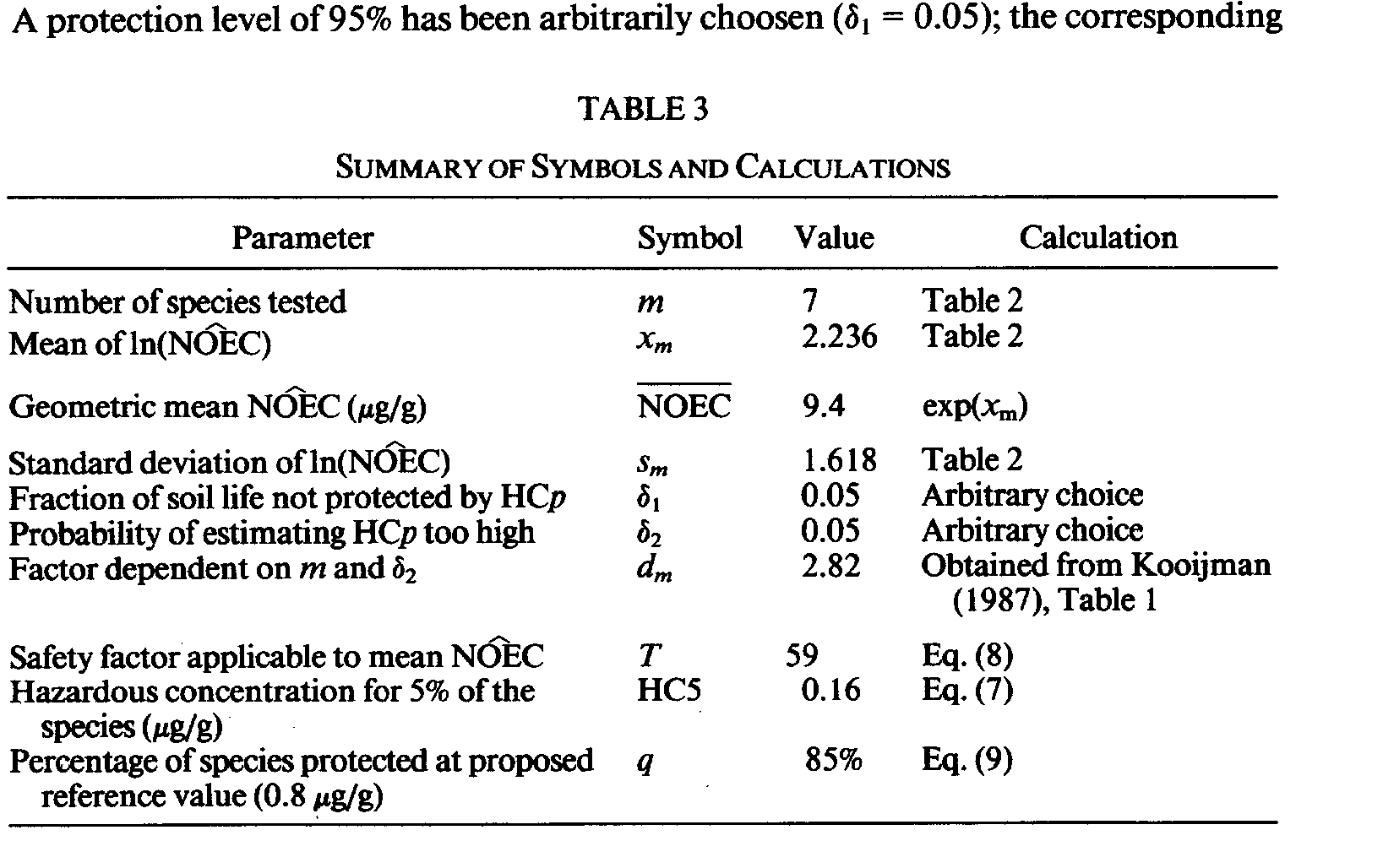
They gave the 95 percent one justification, and it pointed to the US EPA's water guidelines: "In our opinion, a 95% protection level is a reasonable requirement. In the U.S. EPA 'Guidelines for Deriving Water Quality Criteria,' the same criterion is used for calculating the 'Final Acute Value'" (van Straalen & Denneman, 1989).
In a 2002 book, Species Sensitivity Distributions in Ecotoxicology, van Straalen and a co-author explained why their 95 percent version was adopted and Kooijman's most-sensitive-species version was not: "The numerical values derived using the algorithm of Van Straalen were considered more 'reasonable' than Kooijman's; they were usually low, but above background concentrations. This fact contributed greatly to the acceptance of the method" (van Straalen & van Leeuwen, 2002).
In 1989 the Dutch cabinet made the 95 percent goal a national policy. It did so in a paper titled Omgaan met risico's (Premises for Risk Management), which presents the key assumption as provisional (our translation from the Dutch): "it is assumed, for the time being, that the function of the ecosystem is protected if 95 percent of species suffer no adverse effects" ("Daarbij wordt er vooralsnog van uitgegaan dat de functie van het ecosysteem wordt beschermd als er voor 95% van de soorten géén nadelige effekten zijn") (VROM, 1989). The "for the time being" still stands: the 2025 guidance of the Dutch National Institute for Public Health and the Environment (RIVM) says the definition has "been maintained in the Dutch policy on substances over the years." Its limit is still "the concentration which protects at least 95% of the species in an ecosystem" (RIVM, 2025). The same 1989 paper set the human limit of one in a million per year that we discussed in One in a Million.
OECD workshop of 1990
The two lines of work met in December 1990, at a workshop in Arlington, Virginia, run by the Organisation for Economic Co-operation and Development (OECD), an intergovernmental body of industrialized countries. The report says it was "hosted by the United States Environment Protection Agency's Environmental Research Laboratory-Duluth, in co-operation with the Directorate for Chemicals and Risk Management of the Dutch Ministry of Housing, Physical Planning and Environment" (OECD, 1992). The American, Dutch and Danish versions of the method were discussed as one family. The standard reference book on the method, Species Sensitivity Distributions in Ecotoxicology (2002), later credited the meeting with ending "the period of independent development" and wrote that it "originated the term species sensitivity distribution" (Suter, 2002).
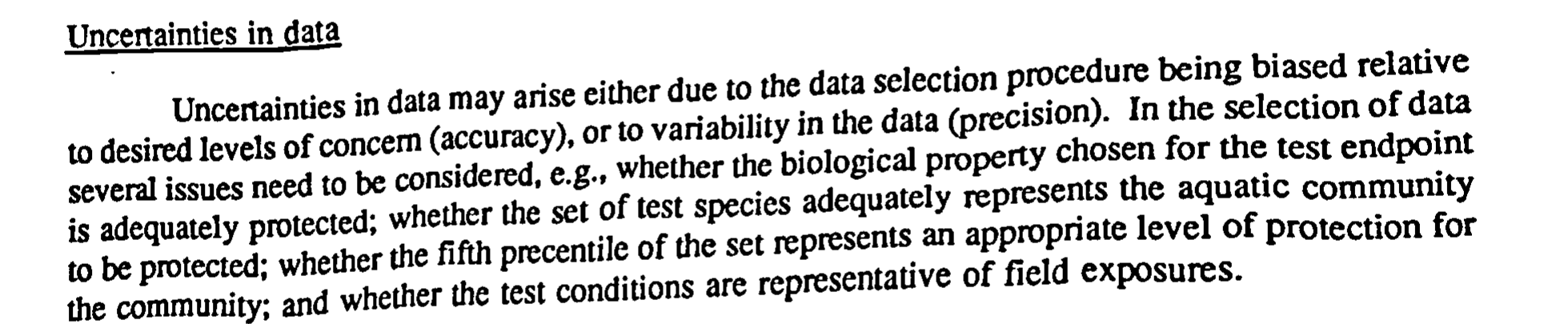
The method's weak points were obvious to the people who formalized and named it. The workshop's report, published in 1992, lists them among the method's uncertainties:
- "whether the biological property chosen for the test endpoint is adequately protected"
- "whether the set of test species adequately represents the aquatic community to be protected"
- "whether the fifth precentile [sic] of the set represents an appropriate level of protection for the community"
- "whether the test conditions are representative of field exposures" (OECD, 1992)
(A test endpoint is the effect a test measures, such as death or slower growth.)
The report also lists checking the method against nature as work still to do: "Validation of extrapolation methods by the use of field studies or mesocosms is recommended" (OECD, 1992). (Mesocosms are outdoor ponds, tanks or artificial streams stocked with several species.)
Does the method hold?
More than thirty-five years on, we can check how well those assumptions have held.
Are the tested species representative of the community?
Regulators do not agree on how many species need to be tested. Two US EPA researchers wrote in 2022 that "there is no consensus among regulatory bodies on the minimum taxonomic data requirements needed to generate a robust SSD." European guidance asks for "at least 10 NOECs (preferably more than 15) for different species covering at least 8 taxonomic groups" (ECHA, 2008). (A NOEC, or "no observed effect concentration," is the highest concentration at which a test found no statistically significant difference from untreated organisms.) Which species are tested matters as much as how many: "the taxonomic composition of the SSD can have a greater influence on HC5 estimates than the number of species" (Dhond & Barron, 2022).
An SSD treats the tested species as a random sample of the community. Van Straalen and Denneman had noted the problem in 1989: "The model assumes that the set of tested species constitutes a random sample from the community to be protected. In practice, species have been selected for quite other reasons (abundance, experimental manageability, interest of researcher)" (van Straalen & Denneman, 1989). In 1993 two ecologists at Denmark's National Environmental Research Institute, T. L. and V. E. Forbes, asked what population those species were a sample of. Their answer:
But how do we know the assumptions are reasonable? The answer is that we do not. There are currently no acute or chronic toxicity data based on random samples from a well-defined ecosystem that can be compared to any of the hypothetical species sensitivity distributions. (Forbes & Forbes, 1993)
In 2002 Valery Forbes and Peter Calow reviewed the SSD studies published in the risk-assessment section of a leading journal, Environmental Toxicology and Chemistry, from 1996 to early 2001. They found that "none of the distributions was a community-SSD despite the fact that a number had site-specific communities as targets of the risk assessment." Such curves, they concluded, "do not represent any known community, but are often interpreted as if they do." When Forbes and Calow rebuilt two published curves so that the mix of plants, invertebrates and fish matched a plausible food web, the fifth percentile moved threefold: down by a factor of 3.4 for cadmium, up by 3.2 for a detergent chemical (Forbes & Calow, 2002).
The author of the EPA's software for fitting these curves shows the problem in one of his examples. His 2020 curve for dichlorodiphenyltrichloroethane (DDT) in birds drew two-thirds of its species from the fowl and waterfowl, a group that, by his figure, makes up about 4.5 percent of bird species (Etterson & Koehrn, 2020).
The EPA has raised most of these objections itself. When it set screening levels for contaminated soil at Superfund sites (polluted locations that require long-term cleanup of hazardous materials), it weighed species curves for birds and mammals and turned them down. It cited the Forbeses' 1993 critique for "the limitations of the distribution-based extrapolation models." It noted that the bird curves had been built from lethal doses, while long-term harm works differently. Citing a 1994 review, the EPA reported that in reproduction tests the two standard birds, the mallard and the bobwhite quail, differed so much that "there was greater similarity between the rat and bird results than between that of the two bird species." (The first essay in this series, Of Mice and Men and Round Numbers, met the same problem: how far one species can stand in for another.) Long-term studies varied so widely in "endpoints, exposure durations, test species, exposure routes, test conditions" that they were "non-comparable and inappropriate for plotting as a distribution." Its main reason for rejecting the curves was "the lack of an adequate toxicological database" (US EPA, 2007).
In its other programmes, the EPA uses the species curves anyway. It currently uses the 1985 guidelines for its national water criteria (US EPA, 2025a). Its pesticide office uses species curves, where available, in reviews of harm to endangered species (US EPA, 2020).
Which curve, and how sure?
There is no biological reason to choose one curve shape over another. The population of species sensitivities, the 1990 workshop stated, "is largely hypothetical and there is no theoretical basis for any particular distribution" (OECD, 1992). Kooijman called his choice of curve "the weakest point" (Kooijman, 1987). Aldenberg and Slob used the same curve because it "has some nice mathematical features that make certain calculations relatively easy" (Aldenberg & Slob, 1993). Even the method of fitting matters. Two statisticians at Durham University took a hypothetical chemical with test values for eight species and applied three standard estimation rules. All three gave the same middle value, 11.37 milligrams per litre. Their fifth percentiles were 0.0438, 0.118 and 0.162 milligrams per litre, nearly fourfold apart (Hickey & Craig, 2012). Our first essay in the series examined the same problem in the tail of human variability.
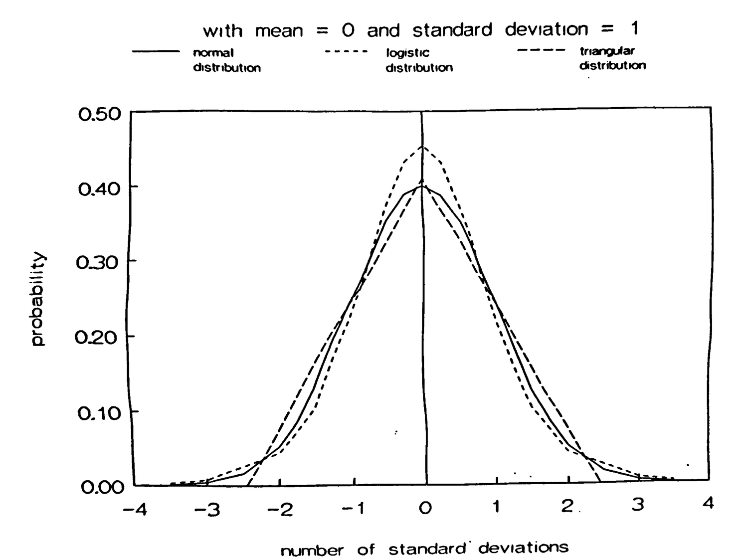
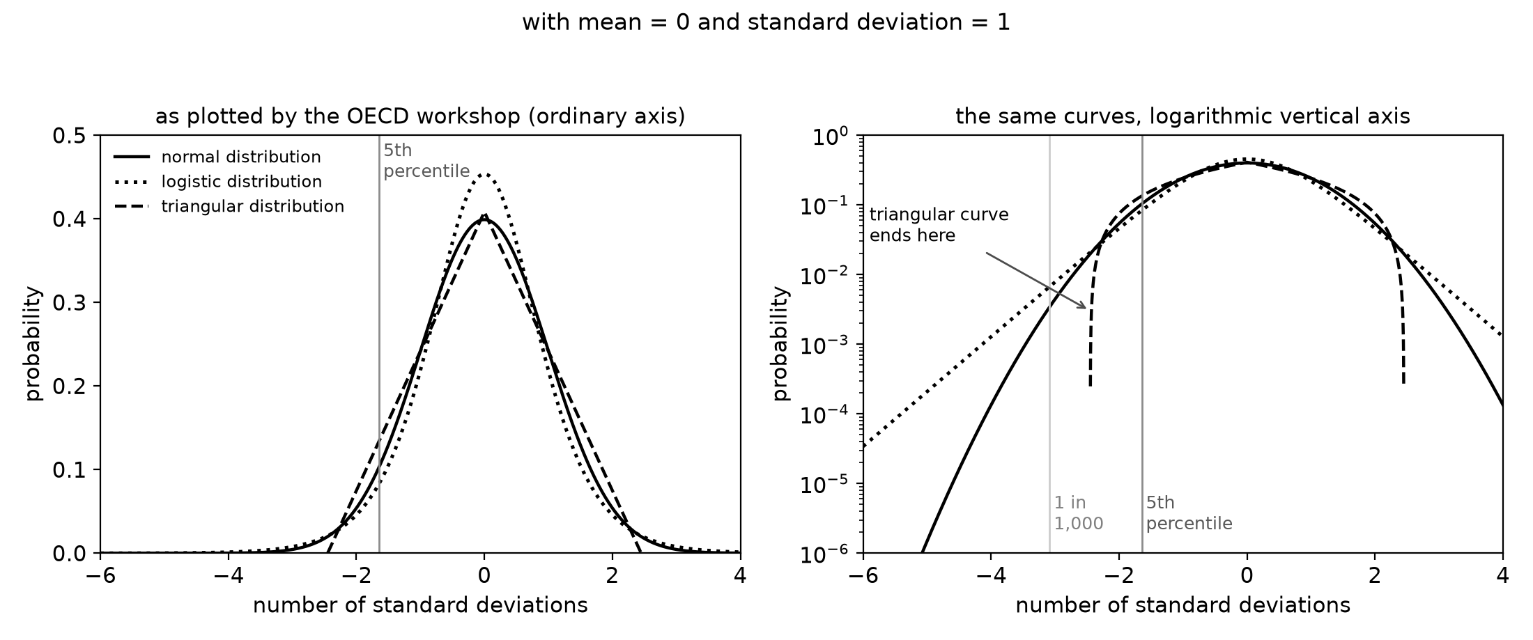
The tail problem was visible from the start. The 1990 workshop drew the three curves then in use (the EPA's triangular, the Danish normal and the Dutch logistic) side by side, with the same average and spread. Plotted the way the report plotted them, they look almost the same. Redrawn with a logarithmic vertical axis, which magnifies small probabilities, the difference is clear. At the fifth percentile the curves still nearly agree. Further out, where Kooijman's threshold sat, they diverge, and the triangular curve simply stops.
Even the scientists who wrote the curve-fitting software agree. In 2021 nine specialists reviewed the state of SSD modelling. Four of them are authors of ssdtools, an open-source package for fitting SSDs that is paid for by the governments of British Columbia, Canada and Australia; its makers say regulators in Canada, Australia and New Zealand use it (CRAN, 2025; Poisson Consulting, 2025). The nine describe the method as "not without numerous limitations," including "the implausibility of the many assumptions underpinning SSDs and concerns arising from inconsistent statistical results." Modelling the left tail, where the fifth percentile sits, "is of critical importance in ecotoxicology, yet in practice this is precisely the region of greatest uncertainty." The usual assumption that one curve fits all the species is, in their words, "invariably false" (Fox et al., 2021).
Which curve an agency picks can drastically change the limit. In 2025 the EPA's chemicals office, with "few reasonably available acute toxicity data" for the solvent 1,1-dichloroethane, built a curve regardless. Two of its four measured values came from tests on a different chemical, and a computer model predicted the rest: "test species (n = 4) and predicted species (n = 75)." The 75 modelled values in that curve of 79 "species" came mostly from the tests on the other chemical. Several curve shapes were then fitted, and one was chosen. The lower bound of that curve's fifth percentile became the agency's threshold for short-term harm to aquatic life (US EPA, 2025b).
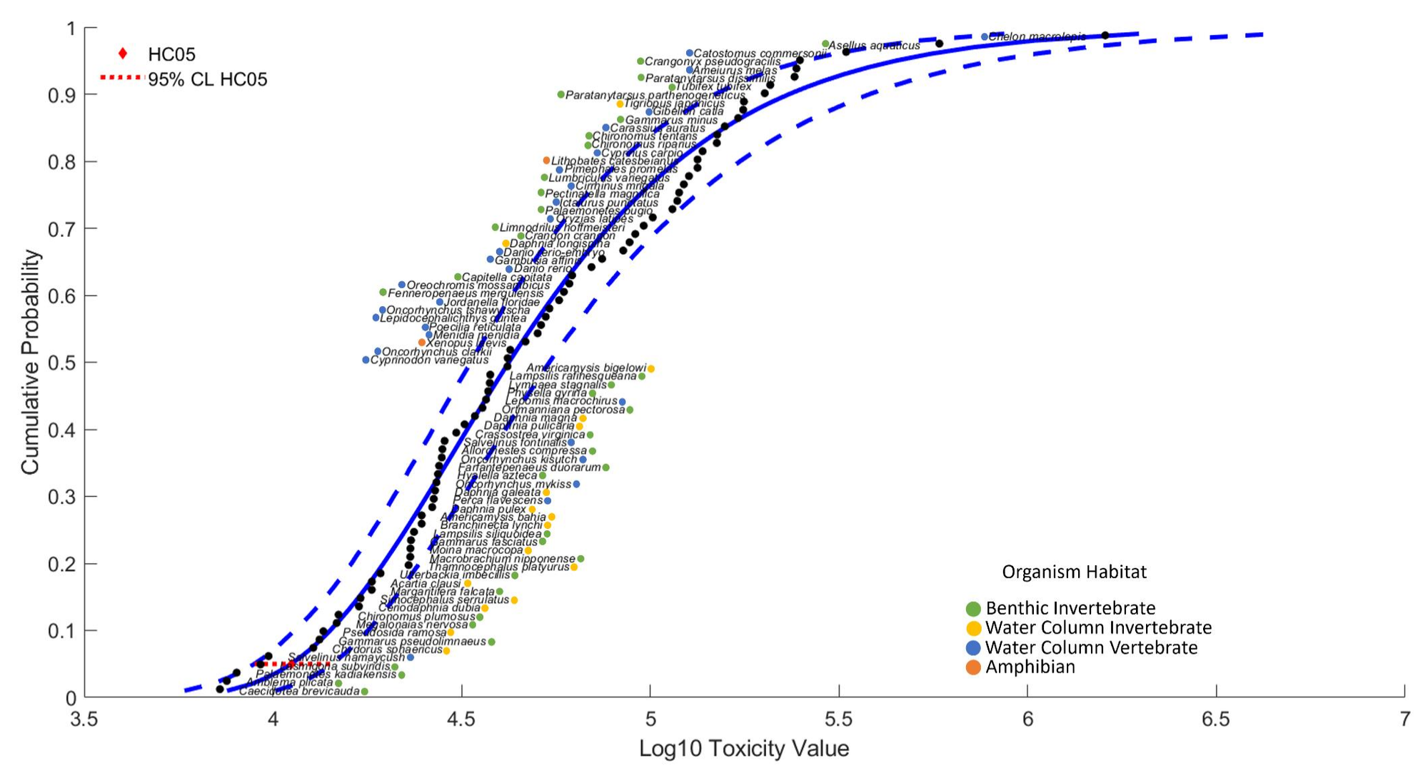
Even with real tests, a fifth percentile estimated from a few species is uncertain, and the 1990 workshop recorded that "there was no consensus on the level of confidence that is appropriate for the protection levels" (OECD, 1992). In 1993 Tom Aldenberg and Wout Slob, statisticians at RIVM (the Dutch National Institute for Public Health and the Environment), offered two versions of the fifth percentile: a cautious lower bound (95 percent confident that the true fifth percentile is no lower), and a middle estimate (as likely to be too high as too low). They warned that "by using the 50% value, one runs the risk of protecting substantially less than 95% of the biological species," and they described what the middle estimate would reward:
On the other hand, using the 50% confidence value as an indication of the safe value results in a strong bias toward economical interests. One would test a minimum number of species, hoping that the coin falls on the right side; if not, one could always extend the number of test organisms afterward. (Aldenberg & Slob, 1993)
Different regulators handle this uncertainty in different ways. The EPA's chemicals office takes the lower bound. European guidance starts from the middle estimate and uses the lower bound only as a check (ECHA, 2008; European Commission, 2018). Australia and New Zealand use the fitted estimate as the guideline value itself, with no confidence limits reported (Warne et al., 2025).
Using the lower bound, however, creates a different incentive. In rejecting the bird and mammal curves, the EPA noted: "As the sample size of the number of species tested increases, the protection threshold also increases" (US EPA, 2007). More species tested means less statistical uncertainty, so the allowed concentration rises. A curve can also replace a safety factor outright, which is a reason to test just enough species to build one. In 2006 a consultant advising 3M on PFOS, one of the "forever chemicals," in birds proposed "egg injection studies with 5 or 6 bird species from which we could derive a species-sensitivity distribution, which could be used to obviate the need for among-species sensitivity factors all together for birds" (Minnesota v. 3M, Ex. 2605).
Is 5 percent the appropriate cut-off?
The HC5 is usually described as the level that protects 95 percent of species. One review of the field puts the convention this way: "to protect 95% of species and, thereby, to accept an adverse effect on 5%" (Spurgeon et al., 2020). Yet the US EPA, which first wrote the fifth percentile into its 1985 guidelines, warned against taking this literally: "Use of 0.05 to calculate a Final Acute Value does not imply that this percentage of adversely affected taxa should be used to decide in a field situation whether a criterion is too high or too low or just right" (US EPA, 1985). Charles Stephan, the guidelines' lead author, wrote that "the 5th percentile applies to a hypothetical population of MAVs, not to MAVs for taxa in any particular field situation" (Stephan, 2002). (A MAV, or mean acute value, is the toxicity figure for one species or genus.) The fifth percentile describes a curve fitted to laboratory results, not the animals living in a river.
The other 95 percent are protected only against an effect large enough for a test to detect. European SSDs are usually built from NOECs (No Observed Effect Concentrations). As we noted in One in a Million, finding no measurable effect can simply mean that the experiment was too small to detect one. Two Australian government scientists, Michael Warne and Rick van Dam, estimated how much harm such tests miss: "The magnitude of the biological effect that NOECs typically cause is 10 to 30%" (Warne & van Dam, 2008). At a typical "no effect" concentration the animals survived, grew or reproduced 10 to 30 percent less than untreated ones.
A NOEC also depends on how the test was run. The 1990 workshop listed the features of a test that shift its NOEC: "the amount of replication, the number and spacing of treatment levels, the variability of the response parameters among replicates, and the precision of the measurements as well as the magnitude of the effects." Fewer animals, widely spaced doses and noisier measurements all make a difference harder to detect, so a small, noisy experiment reports a higher "no effect" level than a more detailed one. The workshop's conclusion: "these endpoints and their distributions have no ecological or biological interpretation" (OECD, 1992).
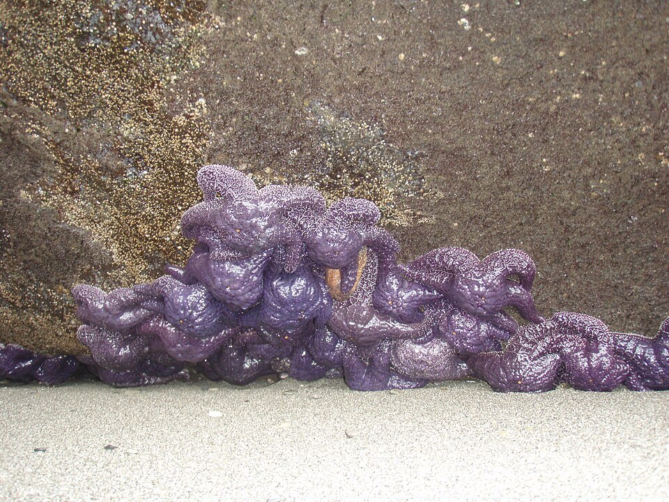
The method does not say which species make up the unprotected 5 percent. The 1990 workshop stated that in these methods "ecosystems are considered to consist of non-interacting species." It assumed that the few species left unprotected "are unlikely to include species that interact with the rest of the ecosystem in important ways (e.g. keystone species)" (OECD, 1992). A keystone species is one whose loss changes the whole community, far out of proportion to its numbers. When the ecologist Robert Paine removed one predatory starfish from a stretch of Pacific shore in the 1960s, the community went "from a 15 to an eight-species system" (Paine, 1966). The workshop gave no evidence for "unlikely." The current EU guidance still says the SSD "is still based on single species data, and species-interactions at the ecosystem level are not covered" (European Commission, 2018). At a 2005 consultation of the EPA's Science Advisory Board (a panel of outside scientists), one panelist noted that "a selected percentile that is statistically defensible might be ecologically unjustifiable" (US EPA SAB, 2006).
Five percent is not the only cutoff in use, either. A 1996 panel on the herbicide atrazine, convened at the request of its maker Ciba-Geigy, which supported the study, chose "the 90th percentile of exposure and 10th percentile of sensitivity." It followed an earlier working group's recommendation and judged these criteria "appropriate for this risk assessment" (Solomon et al., 1996). A 2000 paper by three authors in the same field called the 10th percentile "a conservative indicator of the threshold for effects" and left the acceptable level to the risk manager (Solomon et al., 2000).
Australia and New Zealand openly adjust the percentile to the condition of the ecosystem. Since 2000 their joint water guidelines have published values at "four different protection levels, 99%, 95%, 90% and 80%." The 99 percent values are the default for ecosystems of high conservation value and the 95 percent values for slightly to moderately disturbed ones. For highly disturbed ones the 90 or 80 percent values may be accepted as "intermediate targets for water quality improvement." The choice of level is "the prerogative of each particular state jurisdiction or catchment manager, in consultation with the community and stakeholders." The guidelines support the 95 percent default by precedent: the method "has been adopted in The Netherlands and is recommended by the OECD" (ANZECC & ARMCANZ, 2000).
Are the laboratory measurements representative of the field?
One way to test the method is to compare its predictions with what happens in the field. The 1990 workshop pointed out a limit of that test. A method whose results match observations "verifies that the results are correct without commenting on the appropriateness of the procedures; that is, agreement may be due to counteracting errors" (OECD, 1992). A good match does not, by itself, show that the method's assumptions are right.
Single-species laboratory tests supply the data the species curve is built from. Two kinds of study check the curve against species living together: multi-species experiments in mesocosms, and field studies of real rivers and streams. Most verifications use mesocosms. They are closer to nature than a single-species test, but small, short and simplified.
Researchers at RIVM checked the method against multi-species experiments in 1993, and their conclusion was cautious: "With reservations, due to this paucity of data, it is concluded that single-species toxicity data can be used to derive 'safe' values for the aquatic ecosystem" (Emans et al., 1993).
An influential 1999 comparison by three Procter & Gamble scientists covered 11 substances. It found the laboratory fifth percentile "conservative relative to mean model ecosystem data but … a fairly good predictor of the lower 95% confidence interval on the mean model ecosystem NOEC." The ponds' own "no effect" levels were not low. On average they fell at concentrations "expected to exceed the NOEC of 10 to 52% of genera." The pond studies it pooled were also of different kinds. For copper, some looked only at the film of algae on submerged surfaces and others only at invertebrates. "All are weighted equally in our analysis" (Versteeg et al., 1999).
Later reviews of pond studies are mostly reassuring. A 2016 review of pond and tank studies found that "the output from a laboratory SSD was protective of semifield communities in the majority of studies" (Del Signore et al., 2016). But there are exceptions. For herbicides, "the median acute HC5 is not protective of adverse effects in micro/mesocosms in case of a medium to long-term exposure regime to a herbicide" (Van den Brink et al., 2006). For fungicides, the bare HC5 was protective (below the ponds' no-effect level) for only three of nine chemicals. More cautious estimates were protective for all nine (Maltby et al., 2009). At a 2014 workshop hosted by ECETOC (the European Centre for Ecotoxicology and Toxicology of Chemicals), the chemical industry's research centre, an analysis of pond data for six chemicals found the ponds' own safe levels "generally lower than the HC5," with two exceptions (ECETOC, 2014).
Short experiments also differ from rivers in the concentrations at which effects appear. A 2018 study compared 16 families of stream insects in ten-day stream mesocosm experiments and in a wide field survey, using the metal concentration that reduces abundance by 20 percent. The insects in the experiments tolerated more metal: the ratio of the experimental concentration to the field one ranged from 1.09 to 927, and "81% of these ratios were >10". The authors add that such direct comparisons "should be made with caution" (Iwasaki et al., 2018).
Field studies are rarer, and because they survey existing rivers rather than dosing them, they are observational rather than experimental. They measure chemicals and animals already there, or reuse earlier monitoring data. Sites differ in habitat, nutrients and flow as well as in chemicals, and a survey cannot hold those differences constant. The three below each compare a number taken from a species curve with the animals found in the water.
In a 2011 Colorado study, researchers took 149 samples from Rocky Mountain streams in a mining belt and measured zinc in mayflies. A 20 percent drop in the highest mayfly densities came at 7.0 micrograms of dissolved zinc per litre for the genus Drunella and 3.9 for Rhithrogena. A drop in taxonomic completeness (the taxa found compared with the taxa expected) began at 5.4 micrograms per litre. "These effects on populations and communities occurred at Zn concentrations below the U.S. EPA hardness-adjusted continuous chronic criterion." That criterion is derived by the EPA's 1985 method, which starts from the fifth percentile of genus acute values. It averaged 55 micrograms per litre across the sites, 8 to 14 times above the mayfly thresholds (Schmidt et al., 2011).
In 2014 a team from the Czech Republic and Germany compared SSD predictions with the state of stream invertebrates at sites in Germany, France and Finland, chosen "to minimize the differences in habitat composition." They used a field index that measures the share of pesticide-sensitive species in a stream. The team built six versions of the curves, varying the species included and using either acute data or acute values divided by 10 to approximate chronic (long-term) data. All six ranked the streams well. All six set the 5 percent line too high: the acute curves, the kind "regularly used," by 100 to 1,000 times, and the closest "chronic" version by "more than two times." The authors concluded that the 5 percent threshold "is questionable because it can strongly underestimate the effects on biota" and that their results "caution against defining thresholds based on SSDs alone" (Smetanová et al., 2014).
The most direct test was published in 2025. A team led from the Technical University of Denmark, with co-authors at RIVM, drew on chemical measurements at 5,134 Dutch locations and invertebrate samples at 5,939 locations, matching the 1,286 sites where both existed. For each site, the species curves turn the measured concentrations into a predicted share of species affected. That prediction is compared with the number of sensitive species actually found, relative to the cleanest sites. The study set out to test what it called "no more than a key assumption": that the sensitivities of laboratory-tested species resemble those of species in the field. At the 5 percent policy line, it found "an estimated species loss of approx. 10% at the protective threshold" nationally, and 3 percent in one regional water board, Delfland. Where the curves predicted only 1.7 to 3.7 percent affected, the average loss was already 6.3 percent. The authors wrote: "More than 30 years later, our results show the surprising outcome that the targeted goal of protection is not fully reached" (Oginah et al., 2025).
Why regulators keep it
Regulators keep the method partly because it yields a number from whatever tests happen to exist. Instead of doing more fieldwork when data are missing, regulators treat the gap as a statistical problem. When test data are missing or a limit is questioned, the usual response is more computer modelling and better curve-fitting software rather than more laboratory or field tests. The largest collection now holds curves for 12,386 chemicals. Below the limits derived from them, its authors write, "ecosystems are considered sufficiently protected" (Posthuma et al., 2019).
The push to replace animal tests with computer models, known as "new approach methodologies" (NAMs), goes further: fifth percentiles are now predicted for chemicals that have never been tested. A 2025 paper built models from 3,250 existing toxicity records to predict them, and applied the models to 8,449 industrial chemicals. Its authors grant that SSD modelling is limited by "the scarcity of high-quality, standardized toxicity data across taxa and chemical classes," and that "SSDs alone cannot replace in vivo assays" (Khan et al., 2025). In 2026 a team at RIVM that had built a machine-learning model for the same purpose acknowledged that: "It cannot be presupposed that these models, as currently developed, adequately encompass all possible modes of action. This leads potentially to an underestimation of ecological impacts from chemicals with targeted biological effects." Their model, they concluded, "is in its current form insufficient to fully substitute experimental data for regulatory decision making" (Minnema et al., 2026).
The final limit is rarely the bare fifth percentile. Most regulators divide it by an extra safety factor, and defenders of the method point to that divisor. The 2025 Dutch field study concluded that because the 95 percent criterion "is used in combination with an application factor of 5," the methods "are, on average, serving the set goal" (Oginah et al., 2025). The European Union's 2003 guidance set this assessment factor "between 5 and 1, reflecting the further uncertainties identified," and gave no derivation. The same guidance says of assessment factors in general that they must be used "while not having a strong scientific validity" (European Commission, 2003). The current water guidance makes 5 the default, to cover "residual uncertainty" (European Commission, 2018). The ECETOC workshop heard a proposal for a default of 2 (ECETOC, 2014). The EPA's 1985 guidelines halve the Final Acute Value, so that the limit "will not severely adversely affect too many of the organisms" (US EPA, 1985). Australia and New Zealand apply none (Warne et al., 2025). The divisor thus runs from 1 to 5 depending on the jurisdiction, and only the workshop's 2 was offered with data.
Even the method's defenders do not claim that it has been shown to protect ecosystems. The software specialists quoted above, after all their criticism, still conclude it is worth keeping: "Despite the limitations, SSDs remain a practical tool and, until a demonstrably better inferential framework is available, developments and enhancements to conventional SSD practice will and should continue" (Fox et al., 2021). The editors of the reference book wrote in 2002 that "the assumption that SSD-derived criteria are protective is an open question." Their defence pointed to the method's own acceptance. If SSD-based criteria "are interpreted simply as reasonable and consistent values, their utility is confirmed in that sense by a record of use that has been politically and legally acceptable. That is, if they were not reasonable and consistent, they would be struck down by the courts or replaced due to pressures from industry or environmental advocacy groups" (Suter et al., 2002). But being accepted by courts and interest groups is not the same as protecting 95 percent of species.
No replacement is in sight, either. The EPA has been trying to replace its 1985 guidelines for more than thirty years. In 1992 it said it would propose revised methods "in fiscal year 1993" (US EPA, 1992). It consulted its Science Advisory Board four times between 1993 and 2003, and again in September 2005. The agency's brief to that last panel said it was considering changes "to replace the Species Sensitivity Distribution model used in the 1985 Guidelines." One panelist wrote in his comments: "The species sensitivity distribution approach should be removed from the Criteria" (US EPA SAB, 2006). In 2015 the agency told invited experts that revision would be "a several year effort." In 2016 it scheduled drafts for "late 2017 and mid-2019" (US EPA, 2015; US EPA, 2016). We could find no draft. By 2022 the 1985 method had produced, in the words of two EPA researchers, "only 60 criteria values" in nearly four decades (Dhond & Barron, 2022).
"For the time being"
Building a species sensitivity distribution requires multiple separate choices: which species to test, which curve to fit to the data, which percentile to use as the cutoff, and what safety factor to divide it by. Its makers said plainly that the key ones were arbitrary. Looking back in 2002, van Straalen wrote: "There were no clear reasons why a value of 5 should be chosen; it seemed to be the most logical choice in the light of statistical conventions" (van Straalen & van Leeuwen, 2002).
The questions the 1990 workshop wrote down are still open. The Dutch cabinet's "for the time being" is now thirty-seven years old. After nearly four decades, a temporary assumption has become a permanent policy.
The species sensitivity distribution was built to assess risks to ecosystems. But a very similar logic was later applied to human health, where it is known as the threshold of toxicological concern (TTC): a daily intake below which a chemical is presumed to pose no appreciable risk (Munro et al., 1996). That is the subject of a later essay.
References
Aldenberg, T., & Slob, W. (1993). Confidence limits for hazardous concentrations based on logistically distributed NOEC toxicity data. Ecotoxicology and Environmental Safety, 25, 48–63. https://doi.org/10.1006/eesa.1993.1006
ANZECC & ARMCANZ. (2000). Australian and New Zealand Environment and Conservation Council & Agriculture and Resource Management Council of Australia and New Zealand, Australian and New Zealand Guidelines for Fresh and Marine Water Quality, Volume 1, National Water Quality Management Strategy Paper No. 4, October 2000, pp. 3.4–2 to 3.4–5 and 3.4–11.
Copius Peereboom-Stegeman, J. H. J., & Copius Peereboom, J. W. (1989). The intake of cadmium in the Kempen, an area in the south of The Netherlands. Ecotoxicology and Environmental Safety, 18, 93–108. https://doi.org/10.1016/0147-6513(89)90095-X
CRAN. (2025). ssdtools: Species Sensitivity Distributions, R package DESCRIPTION file, version 2.7.0 of 31 August 2026 (authors J. Thorley, R. Fisher, D. Fox and C. Schwarz; funders listed as the Province of British Columbia, Environment and Climate Change Canada, and the Australian Government Department of Climate Change, Energy, the Environment and Water), https://cran.r-project.org/package=ssdtools.
Del Signore, A., Hendriks, A. J., Lenders, H. J. R., Leuven, R. S. E. W., & Breure, A. M. (2016). Development and application of the SSD approach in scientific case studies for ecological risk assessment. Environmental Toxicology and Chemistry, 35, 2149–2161. https://doi.org/10.1002/etc.3474
Dhond, A. K., & Barron, M. G. (2022). Advancing fifth percentile hazard concentration estimation using toxicity-normalized species sensitivity distributions. Environmental Science & Technology, 56, 17188–17196. https://doi.org/10.1021/acs.est.2c06857
ECETOC. (2014). Estimating toxicity thresholds for aquatic ecological communities from sensitivity distributions, Workshop Report No. 28, §3.8 (A. M. J. Ragas).
ECHA. (2008). European Chemicals Agency, Guidance on information requirements and chemical safety assessment, Chapter R.10.
Emans, H. J. B., et al. (1993). Validation of some extrapolation methods used for effect assessment. Environmental Toxicology and Chemistry, 12, 2139–2154. https://doi.org/10.1002/etc.5620121122
Estes, J. A., & Palmisano, J. F. (1974). Sea otters: their role in structuring nearshore communities. Science, 185, 1058–1060. https://doi.org/10.1126/science.185.4156.1058
Etterson, M., & Koehrn, K. (2020). "Using the SSD Toolbox to account for interspecific variability in toxicity," US EPA presentation, 27 February 2020, slides 5 and 20, https://www.epa.gov/sites/default/files/2020-02/documents/etterson_ccte_cop_27feb2020.pdf
European Commission. (2003). Technical Guidance Document on Risk Assessment, Part II, European Chemicals Bureau, EUR 20418 EN/2, pp. 99 and 105.
European Commission. (2018). Technical Guidance for Deriving Environmental Quality Standards, Common Implementation Strategy for the Water Framework Directive, Guidance Document No. 27 (updated 2018).
Forbes, T. L., & Forbes, V. E. (1993). A critique of the use of distribution-based extrapolation models in ecotoxicology. Functional Ecology, 7, 249–254. https://doi.org/10.2307/2390202
Forbes, V. E., & Calow, P. (2002). Species sensitivity distributions revisited: a critical appraisal. Human and Ecological Risk Assessment, 8, 473–492. https://doi.org/10.1080/10807030290879781
Fox, D. R., van Dam, R. A., Fisher, R., Batley, G. E., Tillmanns, A. R., Thorley, J., Schwarz, C. J., Spry, D. J., & McTavish, K. (2021). Recent developments in species sensitivity distribution modeling. Environmental Toxicology and Chemistry, 40(2), 293–308. https://doi.org/10.1002/etc.4925
Hickey, G. L., & Craig, P. S. (2012). Competing statistical methods for the fitting of normal species sensitivity distributions: recommendations for practitioners. Risk Analysis, 32(7), 1232–1243. https://doi.org/10.1111/j.1539-6924.2011.01728.x
Iwasaki, Y., Schmidt, T. S., & Clements, W. H. (2018). Quantifying differences in responses of aquatic insects to trace metal exposure in field studies and short-term stream mesocosm experiments. Environmental Science & Technology, 52(7), 4378–4384. https://doi.org/10.1021/acs.est.7b06628
Khan, K., Tucker, N., Martin, H.-J., Nair, V. G., Ali, A., Tagorti, G., & Hardy, B. (2025). Species sensitivity distribution modeling for ecotoxicity prediction of industrial chemicals. Science of the Total Environment, 1006, 180875. https://doi.org/10.1016/j.scitotenv.2025.180875
Kooijman, S. A. L. M. (1987). A safety factor for LC50 values allowing for differences in sensitivity among species. Water Research, 21, 269–276. https://doi.org/10.1016/0043-1354(87)90205-3
Maltby, L., Brock, T. C. M., & Van den Brink, P. J. (2009). Fungicide risk assessment for aquatic ecosystems: importance of interspecific variation, toxic mode of action, and exposure regime. Environmental Science & Technology, 43, 7556–7563. https://doi.org/10.1021/es901461c
Minnema, J., Viljanen, M., Rorije, E., Peijnenburg, W. J. G. M., & Wassenaar, P. N. H. (2026). Predicting aquatic species sensitivity distributions using machine learning in a regulatory setting. Chemical Research in Toxicology, 39, 1288–1301. https://doi.org/10.1021/acs.chemrestox.5c00466
Minnesota v. 3M, Ex. 2605. J. Giesy (ENTRIX, Inc.) to D. Bacon (3M), "Follow up to February 2, 2006 meeting (revised memo)," 17 February 2006; State of Minnesota v. 3M Co., Hennepin County District Court, No. 27-CV-10-28862, plaintiff's exhibit 2605, Bates 3MA02513749; copy at the UCSF Industry Documents Library, https://www.industrydocuments.ucsf.edu/docs/zjwd0346/.
Mount, D. I., & Stephan, C. E. (1967). A method for establishing acceptable toxicant limits for fish—malathion and the butoxyethanol ester of 2,4-D. Transactions of the American Fisheries Society, 96(2), 185–193. https://doi.org/10.1577/1548-8659(1967)96%5B185:AMFEAT%5D2.0.CO%3B2
Munro, I. C., Ford, R. A., Kennepohl, E., & Sprenger, J. G. (1996). Correlation of structural class with no-observed-effect levels: a proposal for establishing a threshold of concern. Food and Chemical Toxicology, 34, 829–867. https://doi.org/10.1016/S0278-6915(96)00049-X
OECD. (1992). Report of the OECD Workshop on the Extrapolation of Laboratory Aquatic Toxicity Data to the Real Environment (Arlington, Virginia, 10–12 December 1990), Environment Monograph No. 59.
Oginah, S. A., Posthuma, L., Slootweg, J., Hauschild, M., & Fantke, P. (2025). Calibrating predicted mixture toxic pressure to observed biodiversity loss in aquatic ecosystems. Global Change Biology, 31(6), e70305. https://doi.org/10.1111/gcb.70305
Paine, R. T. (1966). Food web complexity and species diversity. American Naturalist, 100, 65–75. https://doi.org/10.1086/282400
Poisson Consulting. (2025). "ssdtools: Open-Source Software for Water Quality Guidelines," project page, https://www.poissonconsulting.ca/project/ssdtools/.
Posthuma, L., van Gils, J., Zijp, M. C., van de Meent, D., & de Zwart, D. (2019). Species sensitivity distributions for use in environmental protection, assessment, and management of aquatic ecosystems for 12 386 chemicals. Environmental Toxicology and Chemistry, 38(4), 905–917. https://doi.org/10.1002/etc.4373
RIVM. (2025). National Institute for Public Health and the Environment (RIVM), Guidance for the derivation of environmental risk limits: Introduction and definitions, version 2.0 (2025).
Schmidt, T. S., Clements, W. H., Zuellig, R. E., Mitchell, K. A., Church, S. E., Wanty, R. B., San Juan, C. A., Adams, M., & Lamothe, P. J. (2011). Critical tissue residue approach linking accumulated metals in aquatic insects to population and community-level effects. Environmental Science & Technology, 45, 7004–7010. https://doi.org/10.1021/es200215s
Smetanová, S., Bláha, L., Liess, M., Schäfer, R. B., & Beketov, M. A. (2014). Do predictions from species sensitivity distributions match with field data? Environmental Pollution, 189, 126–133. https://doi.org/10.1016/j.envpol.2014.03.002
Solomon, K. R., et al. (1996). Ecological risk assessment of atrazine in North American surface waters. Environmental Toxicology and Chemistry, 15, 31–76. https://doi.org/10.1002/etc.5620150105
Solomon, K., Giesy, J., & Jones, P. (2000). Probabilistic risk assessment of agrochemicals in the environment. Crop Protection, 19, 649–655. https://doi.org/10.1016/S0261-2194(00)00086-7
Spurgeon, D., Lahive, E., Robinson, A., Short, S., & Kille, P. (2020). Species sensitivity to toxic substances: evolution, ecology and applications. Frontiers in Environmental Science, 8, 588380. https://doi.org/10.3389/fenvs.2020.588380
Stephan, C. E. (2002). Use of species sensitivity distributions in the derivation of water quality criteria for aquatic life by the U.S. Environmental Protection Agency. In L. Posthuma, G. W. Suter II, & T. P. Traas (Eds.), Species Sensitivity Distributions in Ecotoxicology (ch. 11). Lewis Publishers / SETAC. https://doi.org/10.1201/9781420032314.ch11
Suter, G. W., II (2002). North American history of species sensitivity distributions. In L. Posthuma, G. W. Suter II, & T. P. Traas (Eds.), Species Sensitivity Distributions in Ecotoxicology (ch. 2). Lewis Publishers / SETAC. https://doi.org/10.1201/9781420032314.ch2
Suter, G. W., II, Traas, T. P., & Posthuma, L. (2002). Issues and practices in the derivation and use of species sensitivity distributions. In L. Posthuma, G. W. Suter II, & T. P. Traas (Eds.), Species Sensitivity Distributions in Ecotoxicology (ch. 21). Lewis Publishers / SETAC.
US EPA SAB. (2006). US EPA Science Advisory Board, "Consultation on a proposed framework for revising the guidelines for deriving water quality criteria for protection of aquatic life," EPA-SAB-CON-06-004, 8 March 2006, pp. 1, 15, C-44, E-5 (consultation meeting of 21 September 2005).
US EPA. (1978). "Water quality criteria: request for comments," 43 Federal Register 21506–21518 (18 May 1978).
US EPA. (1985). C. E. Stephan, D. I. Mount, D. J. Hansen, J. H. Gentile, G. A. Chapman & W. A. Brungs, Guidelines for Deriving Numerical National Water Quality Criteria for the Protection of Aquatic Organisms and Their Uses.
US EPA. (1992). "Water quality standards; establishment of numeric criteria for priority toxic pollutants" (the National Toxics Rule), 57 Federal Register 60848–60923 (22 December 1992), at 60861.
US EPA. (2007). Guidance for Developing Ecological Soil Screening Levels (Eco-SSLs), Attachment 4-5, SOP #6: "Derivation of Wildlife Toxicity Reference Value (TRV)," OSWER Directive 9285.7-55 (November 2003, revised June 2007), pp. 4-3 to 4-4.
US EPA. (2015). L. Wilcut, W. Lehmann & M. Elias, "Updating EPA's Guidelines for Deriving National Recommended Water Quality Criteria," slides for the invited expert meeting of September 2015 (dated 1 December 2015).
US EPA. (2016). "Request for nominations of experts to augment the Science Advisory Board Ecological Processes and Effects Committee to provide advice on methods for deriving water quality criteria for the protection of aquatic life," 81 Federal Register 59621–59622 (30 August 2016).
US EPA. (2020). Revised Method for National Level Listed Species Biological Evaluations of Conventional Pesticides, Office of Pesticide Programs, 12 March 2020, pp. 15–16.
US EPA. (2025a). "Guidelines for Deriving Numerical National Water Quality Criteria for the Protection of Aquatic Organisms and Their Uses," web page, last updated 16 October 2026 (copy saved 12 November 2026), https://www.epa.gov/wqc/guidelines-deriving-numerical-national-water-quality-criteria-protection-aquatic-organisms-and
US EPA. (2025b). Risk Evaluation for 1,1-Dichloroethane, EPA-740-R-25-013, Office of Chemical Safety and Pollution Prevention, June 2025, pp. 116, 130 and 534–541 (Appendix K).
Van den Brink, P. J., Blake, N., Brock, T. C. M., & Maltby, L. (2006). Predictive value of species sensitivity distributions for effects of herbicides in freshwater ecosystems. Human and Ecological Risk Assessment, 12(4), 645–674. https://doi.org/10.1080/10807030500430559
van Straalen, N. M., & Denneman, C. A. J. (1989). Ecotoxicological evaluation of soil quality criteria. Ecotoxicology and Environmental Safety, 18, 241–251. https://doi.org/10.1016/0147-6513(89)90018-3
van Straalen, N. M., & van Leeuwen, C. J. (2002). European history of species sensitivity distributions. In L. Posthuma, G. W. Suter II, & T. P. Traas (Eds.), Species Sensitivity Distributions in Ecotoxicology (ch. 3). Lewis Publishers / SETAC. https://doi.org/10.1201/9781420032314.ch3
Versteeg, D. J., Belanger, S. E., & Carr, G. J. (1999). Understanding single-species and model ecosystem sensitivity: data-based comparison. Environmental Toxicology and Chemistry, 18, 1329–1346. https://doi.org/10.1002/etc.5620180636
VROM. (1989). Ministerie van VROM, Omgaan met risico's (Premises for Risk Management), annex to the National Environmental Policy Plan.
Warne, M. St. J., & van Dam, R. (2008). NOEC and LOEC data should no longer be generated or used. Australasian Journal of Ecotoxicology, 14, 1–5.
Warne, M. St. J., Batley, G. E., van Dam, R. A., Chapman, J. C., Fox, D. R., Hickey, C. W., Stauber, J. L., & Fisher, R. (2025). Method for deriving Australian and New Zealand water quality guideline values for protecting aquatic ecosystems from toxicants – update of 2018 version, 2025, pp. 3 and 32–33.
Water Quality Act. (1965). Public Law 89-234, 79 Stat. 903.